2.5.2 Profile optimisation

The number and position of these new non-zero elements, which originate from the factorisation in C, depend exclusively on the sequence of unknowns. In the present examples (Fig. 2.5-1 to 2.5-3 in Section 2.5.1) the profile of matrix N includes 12 zero-elements. In matrix C (not shown) all elements in the envelope are non-zero. A numbering system where the profile is significantly smaller (Fig. 2.5-4 to 2.5-6) is shown for the same example as follows.

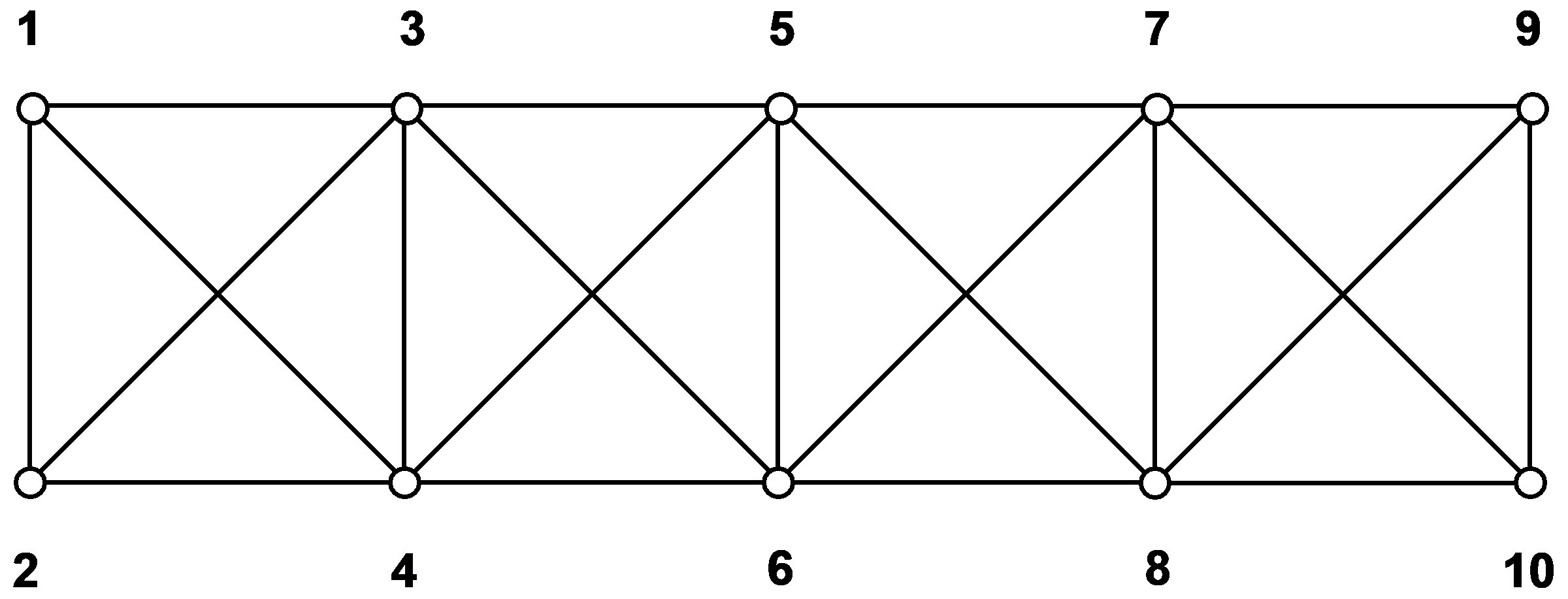
Fig. 2.5-4 Numbering system B

As the necessary memory capacity and computation time may be considerable for larger data blocks, optimisation of the profile is an important task, particularly as the computation effort increases as the square of the size of the profile.

Fig. 2.5-5 Normal-equation matrix and envelope	Fig. 2.5-6 Profile and storage system

In a first step, the photo sequence in the normal equation is optimised according to Banker's algorithm developed by Snay /1976/. In a second step, photo and point unknowns are merged by the program, so that a profile results which is as small as possible /Kruck 1983, 1984/.

The following examples (Fig. 2.5-7 to 2.5-8) illustrate the principles by means of a strip of photos. Additional survey measurements may be added to the matrix without much effect on the profile. For purely geodetic networks a special optimisation is performed because the Banker's algorithm would require too much computing time for this.

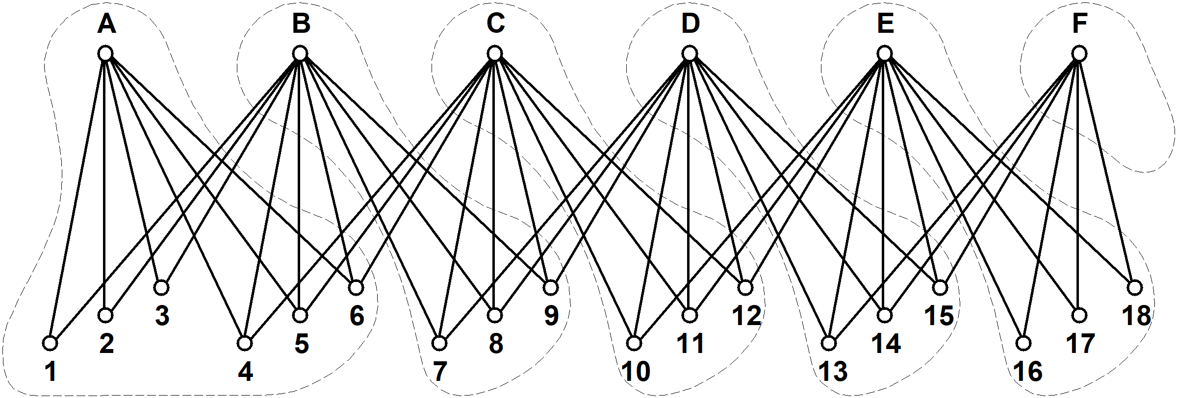
Fig. 2.5-7 Layout of photo strip

Fig. 2.5-8 Normal-equation matrix and envelope of photo strip