2.5.1 Profile storage scheme

Here only a small part of each column is stored in a vector, starting from the first non-zero element in a column to the diagonal element. All these column parts are successively stored in the vector.

A normal equation matrix N according to Fig. 2.5-1 is generated for the network shown in Fig. 2.5-2.
"×" marks the non-zero elements. Fig. 2.5-3 shows the sequence of matrix elements in the computer memory.

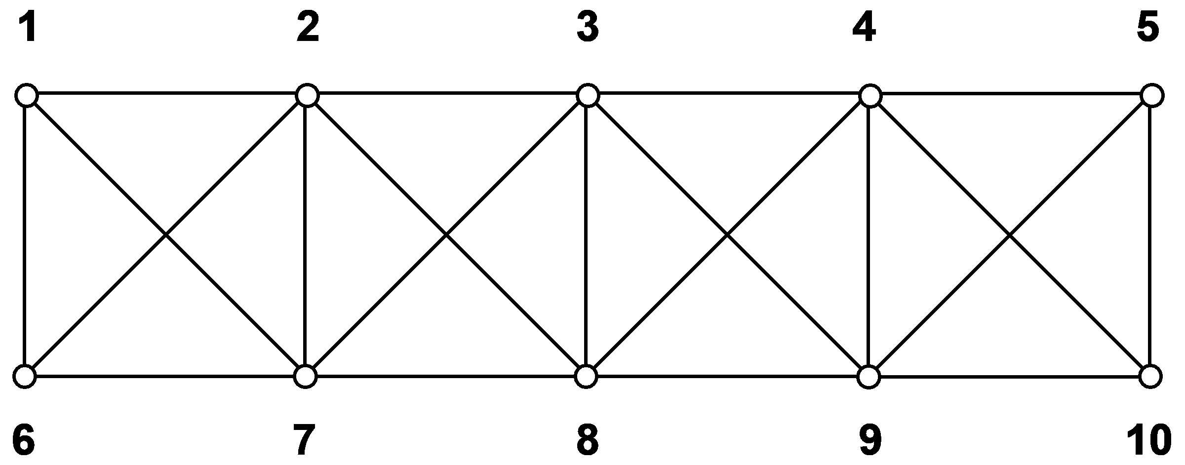
Fig. 2.5-1 Numbering system A

The number of stored elements forms the matrix profile and is included in the envelope. Thus all elements within this envelope are stored, no matter whether they are zero or non-zero. The present example therefore includes several zero elements in the profile.

At least all elements in the matrix C which are non-zero in N are also filled by non-zero elements. C, however, normally includes many more non-zero elements than N, as further non-zero elements result during factorisation according to (2.4/2) (fill-in). These additional elements, however, are always located within the envelope of N.

This is why the matrices N and C are of the same profile. , however, is completely filled with non-zero elements. Here only those elements of will be calculated which are included in the envelope of matrix N (profile inverse). Thus the three matrices, N, C and can be stored similarly.

For very large adjustment tasks the existing core memory is often not sufficient for storage of the entire profile matrix. Therefore, it is divided into blocks, each of which consists of a variable number of columns. These blocks are alternately loaded into the core memory.

The space required for external storage of matrices A, N, C and can roughly be estimated as four times the profile size.

Fig. 2.5-2 Normal-equation matrix and envelope	Fig. 2.5-3 Profile and storage system

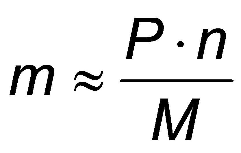
The block lengths and the number of necessary blocks are optimised by the program in order to optimally use the available field length. The minimum number m of blocks is

(2.5.1/1)

with

P :Profile (number of elements in the envelope)

M :Available memory field length

n :A factor between four and five, approximately

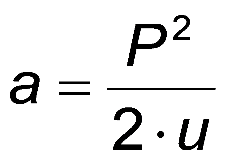
For estimation of the necessary computation time for an adjustment, an average bandwidth is defined:

(2.5.1/2)

with

u :Number of unknowns

The number of necessary multiplications for a factorisation according to (2.4/2) can be estimated for as

(2.5.1/3)

BINGO prints both values in order to give an impression of the computation effort. The approximation equations shown above are not used, however, others which are more precise but much less obvious are used instead.

Equation (2.5.1/3) shows that the computing effort is proportional to the square of the profile value. Therefore, optimisation of the profile is of great importance.

One important advantage of profile storage schemes is the possibility of very fast execution of the tasks "factorisation, computation of solution vector and inversion" on a vector computer. Here a vector computer is to be understood as a computer with special hardware components for fast processing of matrix and vector operations. In most cases, only minor amendments to the program are necessary to address the appropriate hardware components.